---
title: "Running an EWAS with a Snakemake pipeline"
---
```{r}
#| label: setup
#| include: false
source("_setup.R")
```
The previous notebook fit a single association model interactively with `limma`.
Here we introduce using a scalable, reproducible Snakemake pipeline for running
an EWAS. The pipeline automatically handles stratification, meta-analysis, annotation
of results, and basic plotting of results (manhattan and qq plot). In addition, it can
run a differentially methylated region (DMR) analysis. The pipeline utilizes parallelization
and can be run on your local computer or on a remote high performance computing cluster.
The EWAS Snakemake pipeline with installation and run instructions can be found at:
[github.com/krferrier/EWAS](https://github.com/krferrier/EWAS).
We run the whole thing here on the same Grady subset we have been using — the 87
samples with complete covariate data — across the **full filtered probe set**
(756,251 CpGs), the same matrix and the same model chapter 06 fit interactively.
## 1. The pipeline's structure {#sec-structure}
The repository is a standard Snakemake project. The pieces that matter for a
user:
| Path | Role |
|------|------|
| `config.yml` | **The only file you normally edit** — points at your data, names the association variable, toggles stratification / DMR analysis, sets chunking and compute. |
| `Snakefile` + `rules/*.smk` | The DAG: `combined_ewas`, `stratified_ewas`, `dmr`, `annotate`, `plots`. |
| `scripts/ewas.R` | Fits the per-CpG model over a chunk of CpGs; used for both the combined and stratified runs. |
| `scripts/stratify.R` | Splits the methylation + phenotype tables into per-stratum `.fst` files. |
| `scripts/run_bacon.R` | Applies BACON to a results file; writes adjusted stats + diagnostic plots. |
| `scripts/metal_cmd.sh` | Emits a METAL command file from the stratum results. |
| `software/metal/` | METAL source (built once into a binary). |
The dependency graph, conceptually:
```
┌─ combined EWAS ─────────────► BACON ─► plots ─┐
mvals+pheno ┤ ├─► (DMR) ─► annotation
└─ stratify ─► per-sex EWAS ─► BACON ─► METAL ──┘
meta-analysis
```
Because it is Snakemake, running `snakemake --cores N` would build every target
in that graph in dependency order and skip anything already up to date.
## 2. Configuration {#sec-config}
The shipped `config.yml` is annotated for a BMI example; the fields we care about:
```yaml
mvals: data/mvals.csv.gz # CpG × sample M-value matrix (CpGs in rows)
pheno: data/pheno.csv # sample × covariate table; col 1 = sample ID
association_variable: PTSD # the exposure/phenotype to test
stratified_ewas: "yes" # also run within-stratum analyses
stratify_variables: ["sex"] # ...stratified by sex
dmr_analysis: "yes" # region-level analysis after single-CpG
genome_build: hg38 # genome build for annotation
gene_table: refGene
chunk_size: 5000 # CpGs per parallel task
processing_type: cluster # sequential | multisession | multicore | cluster
workers: 4
out_type: ".csv.gz"
```
Notes:
- **`association_variable` is the whole experiment.** Everything else in
`pheno.csv` that is *not* the sample ID or the stratify variable is treated as
a covariate. This is worth internalising: you control the model by choosing
the *columns you write into `pheno.csv`*, not by editing a formula anywhere.
Given the file we build below, the pipeline model is literally
`methylation ~ PTSD + sex + age + smoke + pos + CD8T + CD4T + NK + Bcell + Mono + Neu + SV1 + ... + SV6`
— the same model chapter 06 fit with `limma`, which is what lets us compare
the two implementations at the end of this chapter.
- **`processing_type`** chooses the parallel backend. `cluster` submits chunks as
jobs on an HPC scheduler; on a single machine you use `multicore` or `multisession`. We use
`multicore` below so the demo runs locally.
## 3. Preparing the inputs {#sec-inputs}
The pipeline wants two files: a phenotype file and a methylation data file.
We build them from the preprocessed objects the earlier notebooks produced.
The input file format can be any standard-delimited file type. For the phenotype
file I typically use a .csv or .txt format as the file size is usually relatively
small even without compression. Methylation datasets are typically several GB in size.
I strongly recommend using some form of compression (e.g. `.csv.gz`). You can pass
compressed files to the pipeline without issue. In addition to standardized format types,
like .csv, .txt, etc., you can also use '.fst' filetypes (a fast data serialization format)
which is by far the format type the pipeline can process the fastest.
::: {.callout-note}
## What this chapter needs
Every file this chapter reads lives under `../ewas_pipeline/` and was written by the
pipeline run shown below, not by an earlier chapter. If you have not run the pipeline
yourself, fetch the published run instead:
```{.bash filename="Terminal"}
./get_data.sh G_pipeline_run
```
:::
```{r}
#| label: show-inputs
library(data.table) # fread() for every pipeline output read in this chapter
# The phenotype file the pipeline was given. The paths in this chapter are
# relative to the tutorial folder, so `../ewas_pipeline/` is the pipeline
# checkout sitting beside it -- which is where tier G extracts to.
pheno <- fread("../ewas_pipeline/data/pheno.csv")
cat("pheno.csv:", nrow(pheno), "samples x", ncol(pheno), "columns\n")
cat("columns:", paste(names(pheno), collapse = ", "), "\n\n")
# PTSD is coded 0/1 here rather than Control/Case: ewas.R builds the design from
# the column as it stands, so the coding in this file is the coding modeled.
cat("PTSD (1=Case, 0=Control):\n"); print(table(pheno$PTSD))
cat("\nsex:\n"); print(table(pheno$sex))
```
```r
# mvals.csv.gz — SAMPLES in rows, CpGs in columns, first column = sample IDs.
# This orientation matters: ewas.R moves the first column to rownames and then
# chunks over the *columns*, so the file must be samples x CpGs, not CpGs x samples.
M <- log2((betas + 1e-3) / (1 - betas + 1e-3)) # betas = filtered matrix, probes x samples
M <- M[complete.cases(M), ]
Mt <- t(M)
data.table::fwrite(data.table(SampleID = rownames(Mt), data.table::as.data.table(Mt)),
"data/mvals.csv.gz")
```
This writes the **full filtered probe set** — every CpG that survived chapter 03. The chunking machinery is what makes that affordable: `ewas.R` reads
the matrix once, splits the CpGs into chunks of `chunk-size`, and distributes chunks
across workers, so memory stays flat as the probe count grows.
## 4. Building METAL {#sec-metal-build}
METAL is distributed as C++ source. The pipeline vendors it under
`software/metal/` and builds it once:
```bash
cd software/metal
tar -xzf METAL.tar.gz --strip-components=1
cmake -S . -B build -DCMAKE_BUILD_TYPE=Release
cmake --build build
# → software/metal/build/metal/metal
```
This installation/build is automatically handled by the Snakemake pipeline.
## 5. Running a non-stratified EWAS {#sec-run}
If you don't want to stratify your EWAS by any terms, the pipeline begins
running the EWAS across all 87 complete-data samples with the `ewas.R` script.
This script reads the methylation matrix in chunks, fits one `glm` per CpG, and
uses the `PTSD` term as the main predictor to test for association:
```bash
Rscript scripts/ewas.R \
--pheno data/pheno.csv --methyl data/mvals.csv.gz \
--assoc PTSD --stratified no \
--chunk-size 5000 --processing-type multicore --workers 8 \
--out-dir run_grady_all --out-type .csv.gz
# → run_grady_all/PTSD_ewas_results.csv.gz (756,251 CpGs)
```
On the machine that produced this tutorial — 32 logical cores (24 physical), 126 GB RAM — that took
**5 min 24 s** of EWAS time at 8 workers, and 6 min 12 s including the BACON step that
follows. The two stratified analyses in the next section took 11 min 37 s together at
4 workers each, running concurrently. [Setup](00_setup.qmd) has the memory figures and
guidance on choosing `workers` for your own machine.
### Does the pipeline agree with chapter 06?
Chapter 06 fit this model with `limma::lmFit` + `eBayes`; the
pipeline fits one `glm` per CpG. On this run:
- **Effect estimates are identical** — the largest disagreement between the
pipeline's `estimate` and limma's `logFC` across all 756,251 CpGs is
8.9 × 10⁻¹⁵, i.e. floating-point noise. Same design matrix, same least-squares
solution.
- **Both reference the same *t* distribution** with 63 residual degrees of
freedom.
- **The p-values still differ slightly** (correlation 0.999 on the −log₁₀ scale;
λ = 1.022 from `limma` against 1.021 from the pipeline). The reason is `eBayes`: limma shrinks each probe's
residual variance toward a prior fitted across all probes, so its standard
errors differ from the per-probe `glm` ones by up to ~22%. Neither is wrong,
which highlights the importance of being transparent about which method is used.
Identical point estimates plus a small, explainable difference in the variance
model gives confidence that the results we are seeing are not an artifact of the
method used for association testing.
```{r}
#| label: load-all
# The non-stratified arm, straight out of the ewas.R call above: one row per
# CpG with the per-probe glm estimate, its standard error, the t-statistic and
# the p-value. These are the pre-BACON numbers; the BACON-adjusted file that
# section 7 reads is a separate output of the same run.
allres <- fread("../ewas_pipeline/run_grady_all/PTSD_ewas_results.csv.gz")
cat("columns:", paste(names(allres), collapse = ", "), "\n")
cat("n CpGs:", nrow(allres), " | samples per model (n):", allres$n[1], "\n")
setorder(allres, p.value)
print(head(allres[, .(cpgid, estimate, std.error, statistic, p.value)], 5))
```
## 6. Stratifying by sex, then running each stratum {#sec-strata}
If you want to run a stratified EWAS, you first run `stratify.R` on your variable(s)
that you'd like to stratify by. The script splits both the phenotype and methylation
tables by the stratify variable(s) and drops that variable from the phenotype file before
being passed on to the EWAS step.
```bash
Rscript scripts/stratify.R --stratify sex --out-dir run_grady --threads 4
# → run_grady/F/{F_mvals.fst, F_pheno.fst}
# → run_grady/M/{M_mvals.fst, M_pheno.fst}
for S in F M; do
Rscript scripts/ewas.R \
--pheno run_grady/$S/${S}_pheno.fst \
--methyl run_grady/$S/${S}_mvals.fst \
--assoc PTSD --stratified yes \
--chunk-size 5000 --processing-type multicore --workers 4 \
--out-dir run_grady/$S --out-prefix $S --out-type .csv.gz
done
# → run_grady/F/F_PTSD_ewas_results.csv.gz (n = 45)
# → run_grady/M/M_PTSD_ewas_results.csv.gz (n = 42)
```
The female stratum has 45 samples, the male 42. Each within-stratum model is now
`methylation ~ PTSD + age + cell composition`.
## 7. BACON: correcting residual inflation and bias {#sec-bacon}
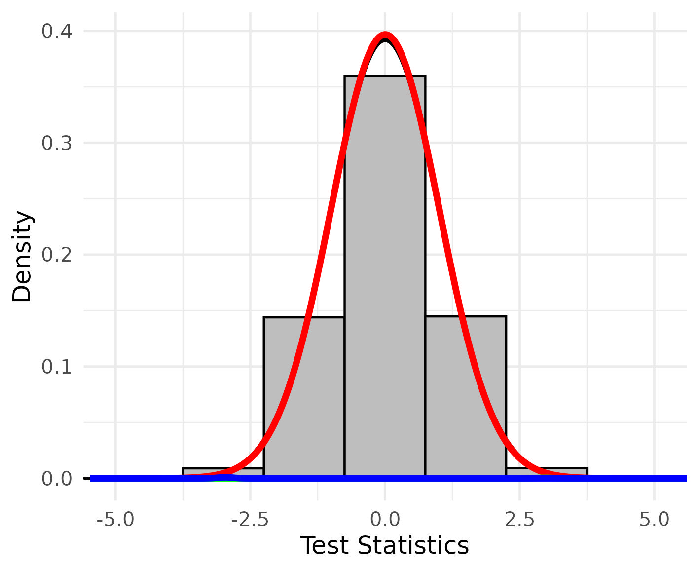
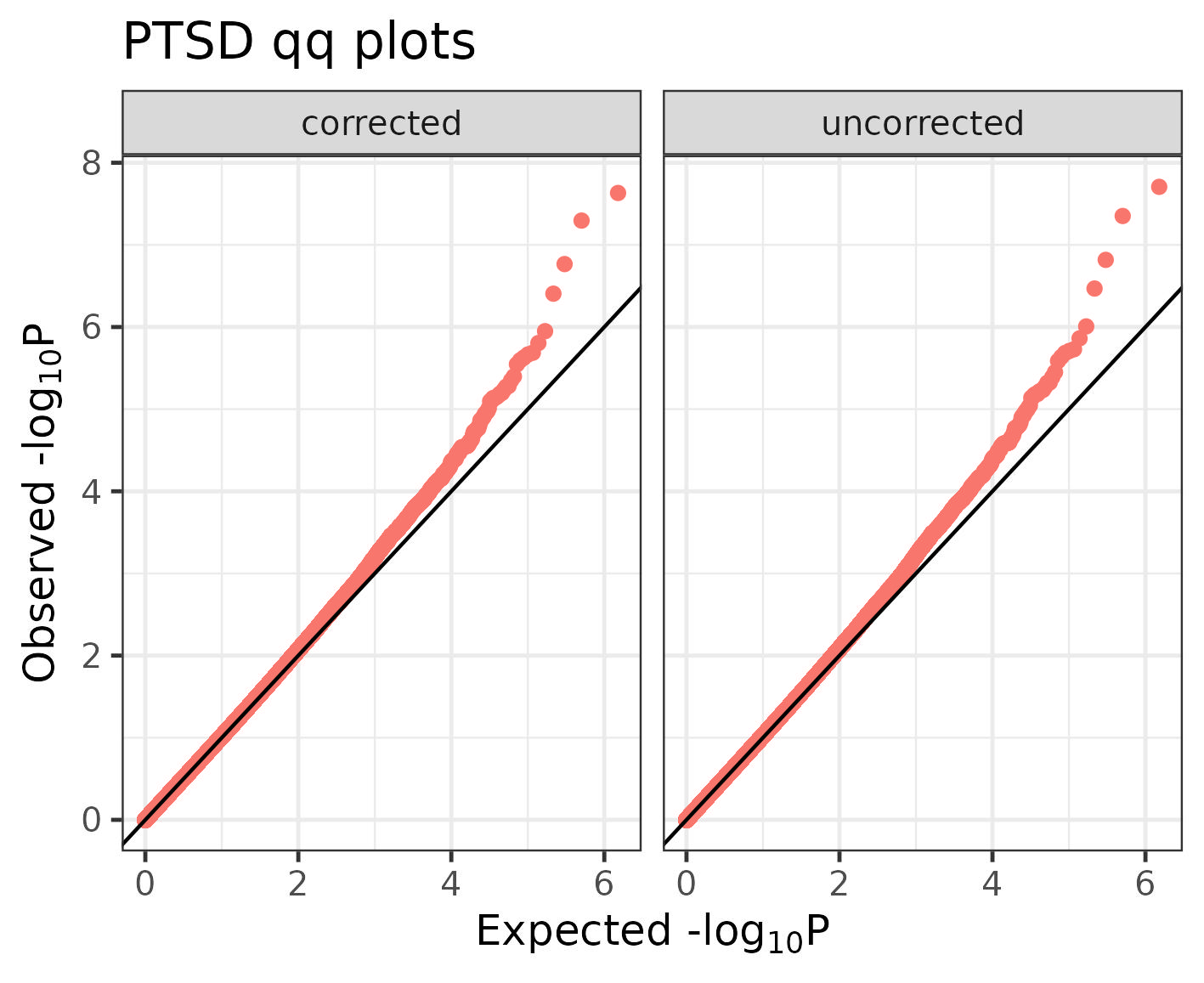
A well-specified EWAS should have a genomic-inflation factor `λ ≈ 1` and a QQ
plot on the diagonal until the extreme tail. In practice small-sample EWAS often
show *deflation* (`λ < 1`) or a slight bias in the test-statistic distribution
that covariate adjustment does not fix. **BACON** [@vanIterson2017bacon] fits a
three-component Gaussian mixture to the test statistics by Gibbs sampling,
estimates the bias (mean) and inflation (SD) of the *null* component, and rescales
every statistic accordingly. The pipeline runs it on each analysis (or just the output
EWAS results if no stratification is done):
```bash
for S in F M; do
Rscript scripts/run_bacon.R \
-i run_grady/$S/${S}_PTSD_ewas_results.csv.gz \
--out-dir run_grady/$S --out-prefix $S --out-type .csv.gz
done
# the combined arm, whose output carries no group prefix
Rscript scripts/run_bacon.R \
-i run_grady_all/PTSD_ewas_results.csv.gz \
--out-dir run_grady_all --out-type .csv.gz
```
`run_bacon.R` uses fixed priors and seeds (`niter = 5000`, `nburnin = 2000`,
`globalSeed = 42`) so the correction is reproducible, and it writes four
diagnostic plots per analysis (mixture fit, MCMC traces, posteriors, and a
before/after QQ). It appends `bacon.pval`, `bacon.es`, `bacon.se`,
`bacon.statistic`, and the pre/post `lambda`/`b.lambda` to the results.
Here is what BACON did to the genomic inflation in each arm:
```{r}
#| label: lambda-table
# Genomic inflation: the median observed chi-square over its null expectation.
# Zero and non-finite p-values are dropped first -- METAL writes a handful of
# exact zeros at the extreme tail, and qchisq() would return Inf for those.
lam <- function(p) { p <- p[is.finite(p) & p > 0]
median(qchisq(p, 1, lower.tail = FALSE)) / qchisq(0.5, 1) }
# The four arms. Each BACON results file carries both the raw `p.value` and the
# adjusted `bacon.pval`, which is what lets one row report lambda before and
# after the correction. Reading all four costs ~160 MB of compressed CSV.
res_all <- fread("../ewas_pipeline/run_grady_all/PTSD_ewas_bacon_results.csv.gz")
res_f <- fread("../ewas_pipeline/run_grady/F/F_PTSD_ewas_bacon_results.csv.gz")
res_m <- fread("../ewas_pipeline/run_grady/M/M_PTSD_ewas_bacon_results.csv.gz")
# The METAL table is read again in section 8, where the chapter works through
# its columns; here only its p-values are needed.
res_meta <- fread("../ewas_pipeline/run_grady/PTSD_ewas_meta_analysis_results_1.txt")
setnames(res_meta, "P-value", "P")
# One row per EWAS arm. `n` comes out of the results file itself: ewas.R records
# the number of samples that entered each per-CpG model.
row1 <- function(lab, d) {
setorder(d, bacon.pval)
data.table(Analysis = lab, n = d$n[1],
lambda_raw = lam(d$p.value), lambda_bacon = lam(d$bacon.pval),
n_P_lt_1e5 = sum(d$bacon.pval < 1e-5, na.rm = TRUE),
top_cpg = d$cpgid[1], top_P = d$bacon.pval[1])
}
# The meta-analysis row is built by hand rather than through row1(): METAL's
# output has no per-CpG sample size and no uncorrected p-value to compare
# against, because its inputs were already BACON-adjusted.
summ <- rbindlist(list(
row1("Overall", res_all), row1("Female", res_f), row1("Male", res_m),
data.table(Analysis = "Meta (F+M)", n = NA_integer_,
lambda_raw = NA_real_, lambda_bacon = lam(res_meta$P),
n_P_lt_1e5 = sum(res_meta$P < 1e-5, na.rm = TRUE),
top_cpg = res_meta$MarkerName[which.min(res_meta$P)],
top_P = min(res_meta$P))))
# Small and rectangular, so it goes in the repository as a flat file: a reader
# who cannot hold four 756,251-row tables in memory can still read this table.
fwrite(summ, "data/07_pipeline_summary.csv")
print(summ[, .(Analysis, n, lambda_raw = round(lambda_raw, 3),
lambda_bacon = round(lambda_bacon, 3),
n_P_lt_1e5, top_cpg, top_P = signif(top_P, 3))])
```
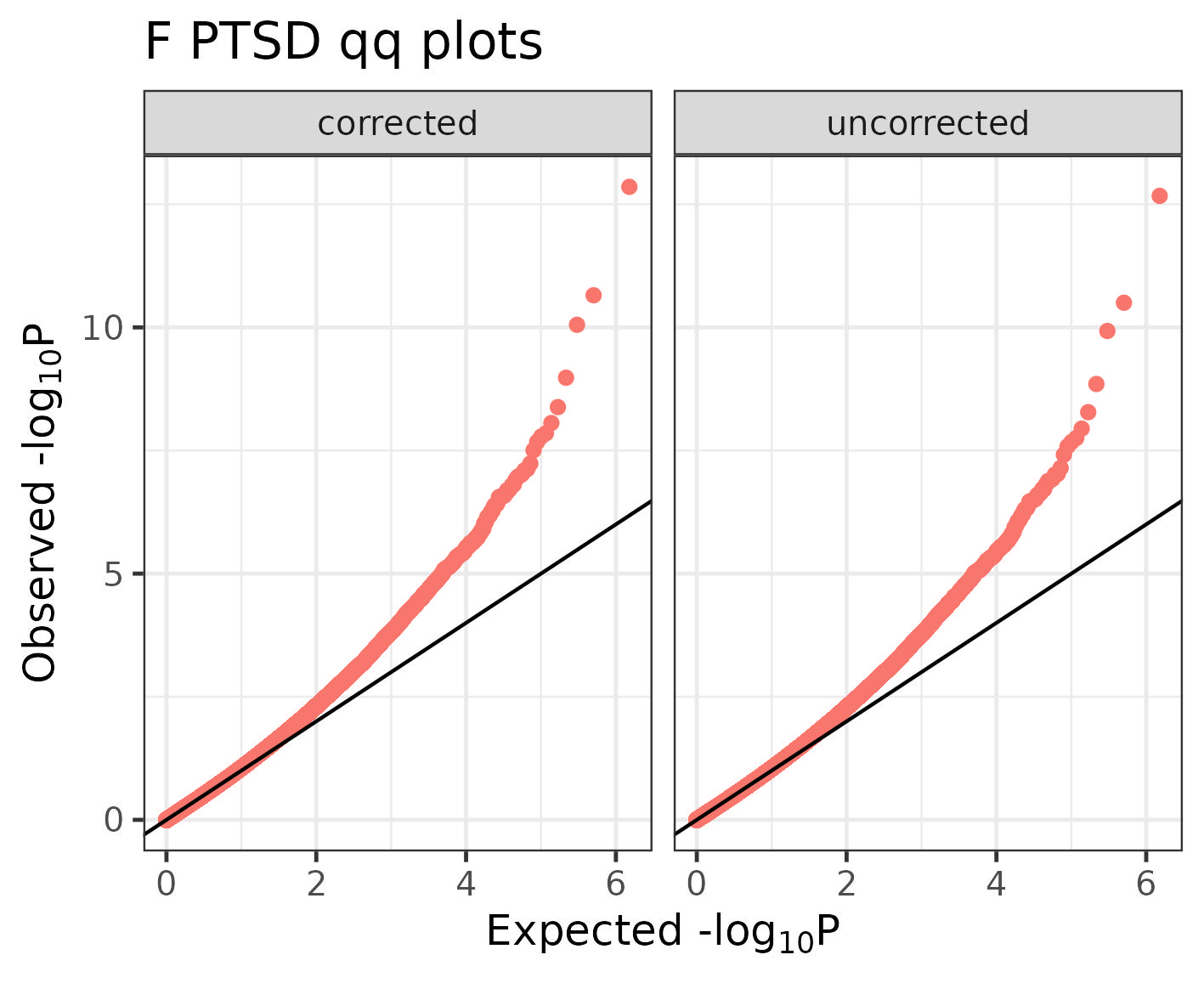
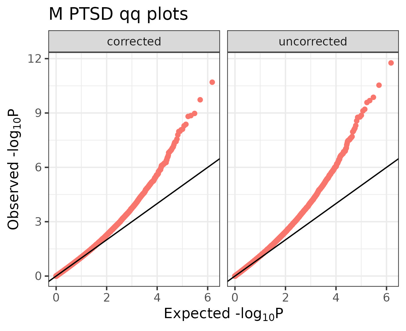
The raw λ values start close to 1 but pull in *opposite directions* across the
strata: 1.021 in the combined arm, 0.967 in females (mildly deflated), 1.070 in
males (mildly inflated). BACON pulls all three to within 2.5% of 1.0 — 1.023 /
1.014 / 1.013 — which is the behavior you want from it: a small, symmetric
correction of residual bias, not a rescue of a badly specified model.
Note that the male arm needed the largest correction. With 42 samples and the
same covariate count, it has the least residual signal to estimate a variance
from, so its test statistics are the most over-dispersed to begin with. This is
the general pattern in stratified EWAS — the smaller stratum is the more likely
the λ is to be in- or de-flated.
The mixture fit and the before/after QQ for the overall analysis:
```{r}
#| label: copy-bacon-plots
# run_bacon.R already drew these four; copying them in under the names the
# figures below use is honest provenance and avoids redrawing a plot from a
# sampler that has already been run. The pipeline writes them per analysis, so
# the overall arm's files carry no group prefix and the strata do.
dir.create("data/07_bacon", showWarnings = FALSE, recursive = TRUE)
invisible(file.copy(
c("../ewas_pipeline/run_grady_all/bacon_plots/PTSD_fit.jpg",
"../ewas_pipeline/run_grady_all/bacon_plots/PTSD_qqs.jpg",
"../ewas_pipeline/run_grady/F/bacon_plots/F_PTSD_qqs.jpg",
"../ewas_pipeline/run_grady/M/bacon_plots/M_PTSD_qqs.jpg"),
c("data/07_bacon/all_fit.jpg", "data/07_bacon/all_qqs.jpg",
"data/07_bacon/F_qqs.jpg", "data/07_bacon/M_qqs.jpg"),
overwrite = TRUE))
```
::: {layout-ncol=2}
{#fig-bacon-fit}
{#fig-bacon-qq}
:::
The two stratum QQs after correction:
::: {layout-ncol=2}
{#fig-f-qq}
{#fig-m-qq}
:::
::: {.callout-important}
## BACON is not an excuse to ignore λ
BACON corrects the *distribution* of test statistics; it does not manufacture
signal. If your λ is inflated because of unmodeled batch or cell composition,
the right response is to fix the model (chapters 04 and 05), not to lean on BACON. Use it for
the residual bias that remains after adjustment.
:::
## 8. Meta-analyzing the strata with METAL {#sec-meta}
Now we combine the two sex-specific results with **METAL** [@willer2010metal].
Because the pipeline wrote its columns with the labels METAL expects, generating the
command file is simple:
```bash
bash scripts/metal_cmd.sh \
run_grady/meta_analysis/PTSD_metal_commands.txt \
run_grady/meta_analysis/PTSD_ewas_meta_analysis_results_ \
run_grady/F/F_PTSD_ewas_bacon_results.csv.gz \
run_grady/M/M_PTSD_ewas_bacon_results.csv.gz
software/metal/build/metal/metal run_grady/meta_analysis/PTSD_metal_commands.txt
```
The generated command file tells METAL to run an **inverse-variance** (`SCHEME
STDERR`) meta-analysis, reading the **BACON-adjusted** effect, SE, and p-value
columns, weighting by `n`, and testing for **heterogeneity** across the sexes:
```
SCHEME STDERR
SEPARATOR COMMA
PVALUELABEL bacon.pval
EFFECTLABEL bacon.es
STDERRLABEL bacon.se
MARKER cpgid
WEIGHT n
PROCESSFILE .../F_PTSD_ewas_bacon_results.csv.gz
PROCESSFILE .../M_PTSD_ewas_bacon_results.csv.gz
ANALYZE HETEROGENEITY
```
```{r}
#| label: load-meta
# METAL's output table, one row per CpG present in both strata. The `_1` suffix
# is METAL's own: it numbers the analyses in a command file, and this run has
# one. Column names come from METAL, hence the backticks around `P-value`.
meta <- fread("../ewas_pipeline/run_grady/PTSD_ewas_meta_analysis_results_1.txt")
setorder(meta, `P-value`)
cat("markers meta-analyzed:", nrow(meta), "\n\n")
print(head(meta[, .(MarkerName, Effect, StdErr, `P-value`, Direction,
HetISq, HetPVal)], 6))
```
Output columns from METAL to note:
- **`Direction`** is one character per input file (`F` then `M`). `++` or `--`
means the effect pointed the same way in both sexes; `+-` or `-+` means it
flipped. The top hit **cg22671410** is `+-`, P = 2.0×10⁻¹³ — and that mismatch
between a tiny p-value and a discordant direction signifies that there may be a
true difference in effect for that CpG across sexes.
- **`HetISq` / `HetPVal`** quantify how much the two strata *disagree*.
A large `HetISq` with small `HetPVal` flags a CpG whose PTSD association differs
by sex. In a model where both sexes are combined, this signal would be missed.
::: {.callout-warning}
The sample sizes of each strata are quite small for an EWAS, so these results
should be interpreted with caution and replicated in a larger subset (or the full
cohort) before any real conclusions about sex-specific signals can be made.
:::
Nine CpGs clear Bonferroni in the meta-analysis. **Eight of the nine are driven
by one stratum alone**, with the other stratum's p-value above 0.05:
| CpG | Direction | Meta P | Female P | Male P | HetI² |
|---|---|---|---|---|---|
| cg22671410 | `+-` | 2.0×10⁻¹³ | 1.4×10⁻¹³ | 0.91 | 0.0 |
| cg03126377 | `++` | 1.4×10⁻¹⁰ | 2.2×10⁻¹¹ | 0.79 | 72.7 |
| cg08002657 | `--` | 4.2×10⁻¹⁰ | 0.32 | 1.9×10⁻¹⁰ | 61.7 |
| cg25298683 | `--` | 3.7×10⁻⁹ | 8.9×10⁻¹¹ | 0.97 | 86.3 |
| cg08907819 | `++` | 3.9×10⁻⁹ | 0.059 | 5.1×10⁻⁹ | 67.2 |
| cg12248040 | `++` | 2.2×10⁻⁸ | 0.22 | 1.1×10⁻⁹ | 86.4 |
| cg09473383 | `++` | 2.9×10⁻⁸ | 9.5×10⁻⁸ | 0.050 | 34.5 |
| cg21102739 | `--` | 3.1×10⁻⁸ | 1.1×10⁻⁷ | 0.11 | 0.0 |
| cg24256418 | `-+` | 4.4×10⁻⁸ | 4.2×10⁻⁹ | 0.78 | 78.5 |
Inverse-variance meta-analysis is a *weighted average*, not a concordance test.
A single stratum with a large effect and a small SE can carry the pooled estimate
past a genome-wide threshold on its own, and the pooled p-value says nothing
about whether the second stratum agreed. Only `cg09473383` is nominally
significant in both arms with matching sign, and it clears 0.05 in the male stratum by
the thinnest possible margin (P = 0.0499) — so even the one apparent replication here is
not something to lean on.
This is why you read `Direction` and `HetISq` alongside `P-value`. Two tips:
1. **Check the arms.** For every hit you plan to report, look up the per-stratum
estimate, SE, and p-value. If one arm is flat, you have a stratum-specific
finding and you should describe it that way.
2. **Distrust `HetISq` at *k* = 2.** With two studies and one heterogeneity
degree of freedom, I² is extremely noisy. `cg22671410` has I² = 0.0 despite
effects of +0.40 and −0.06, because the male SE is so large (0.51) that the
two estimates are statistically compatible with each other. Low I² here means
"not enough precision to tell them apart", not "they agree". That doesn't mean
the results aren't meaningful, they may be an indication of a true sex
difference worth investigating with a more suitable statistical method.
```{r}
#| label: meta-summary
# Same genomic-inflation function as the summary table above, restated so this
# chunk stands on its own if you run it in isolation.
lam <- function(p){p<-p[is.finite(p)&p>0]; median(qchisq(p,1,lower.tail=FALSE))/qchisq(0.5,1)}
cat("meta genomic inflation lambda:", round(lam(meta$`P-value`), 3), "\n")
cat("CpGs with heterogeneity P < 0.05:",
sum(meta$HetPVal < 0.05, na.rm = TRUE),
sprintf("(%.1f%% — right at the 5%% null expectation)\n",
100 * mean(meta$HetPVal < 0.05, na.rm = TRUE)))
```
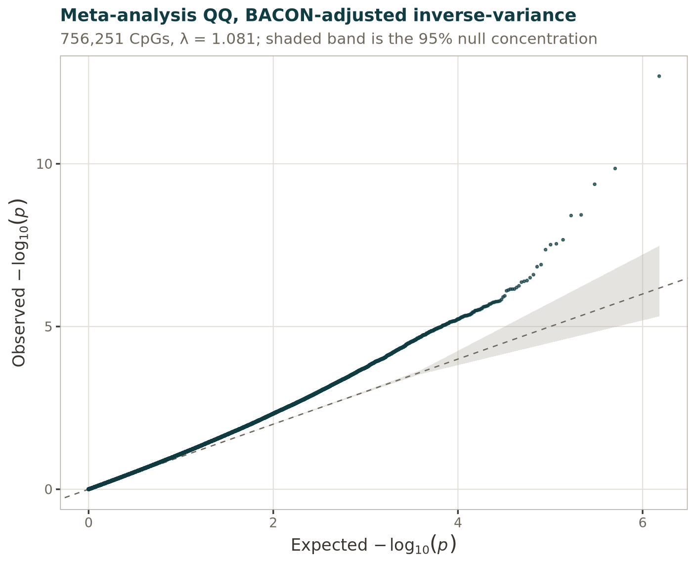{#fig-meta-qq width=70%}
## 9. Reading the run as a whole {#sec-reading}
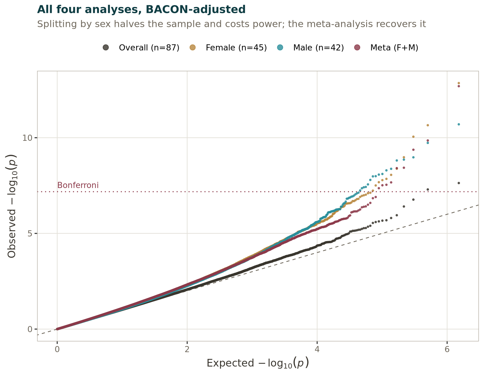
For the purposes of this tutorial, we ran the EWAS with and without stratification, so
we show results for: an 'overall' EWAS model where sex is a covariate, female-only, male-only,
and sex-combined by meta-analysis:
{#fig-qq-overlay width=75%}
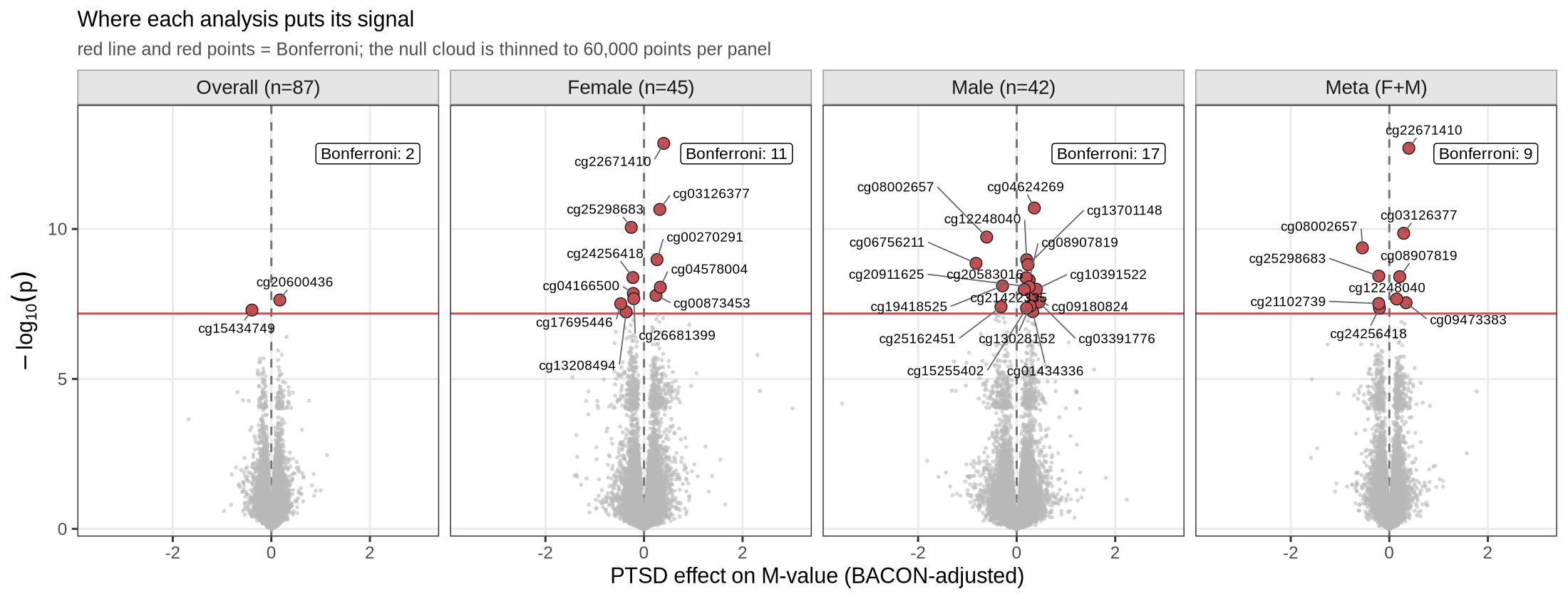
The QQ plots show *how much* signal each analysis reports, but not *where* it sits or
whether the analyses agree. A faceted volcano answers the first question — effect
size against significance, one panel per analysis, on shared axes so the panels are
directly comparable:
{#fig-volcano-facets}
One feature stands out immediately. The stratified arms report far more Bonferroni hits (11 and 17)
than the combined arm (2), despite having roughly half the samples each. While
it is possible some of these are true-positive signals, the small sample size and evidence of poor-fit
prior to BACON adjustment point towards these results being spurious or an artifact of the BACON adjustment.
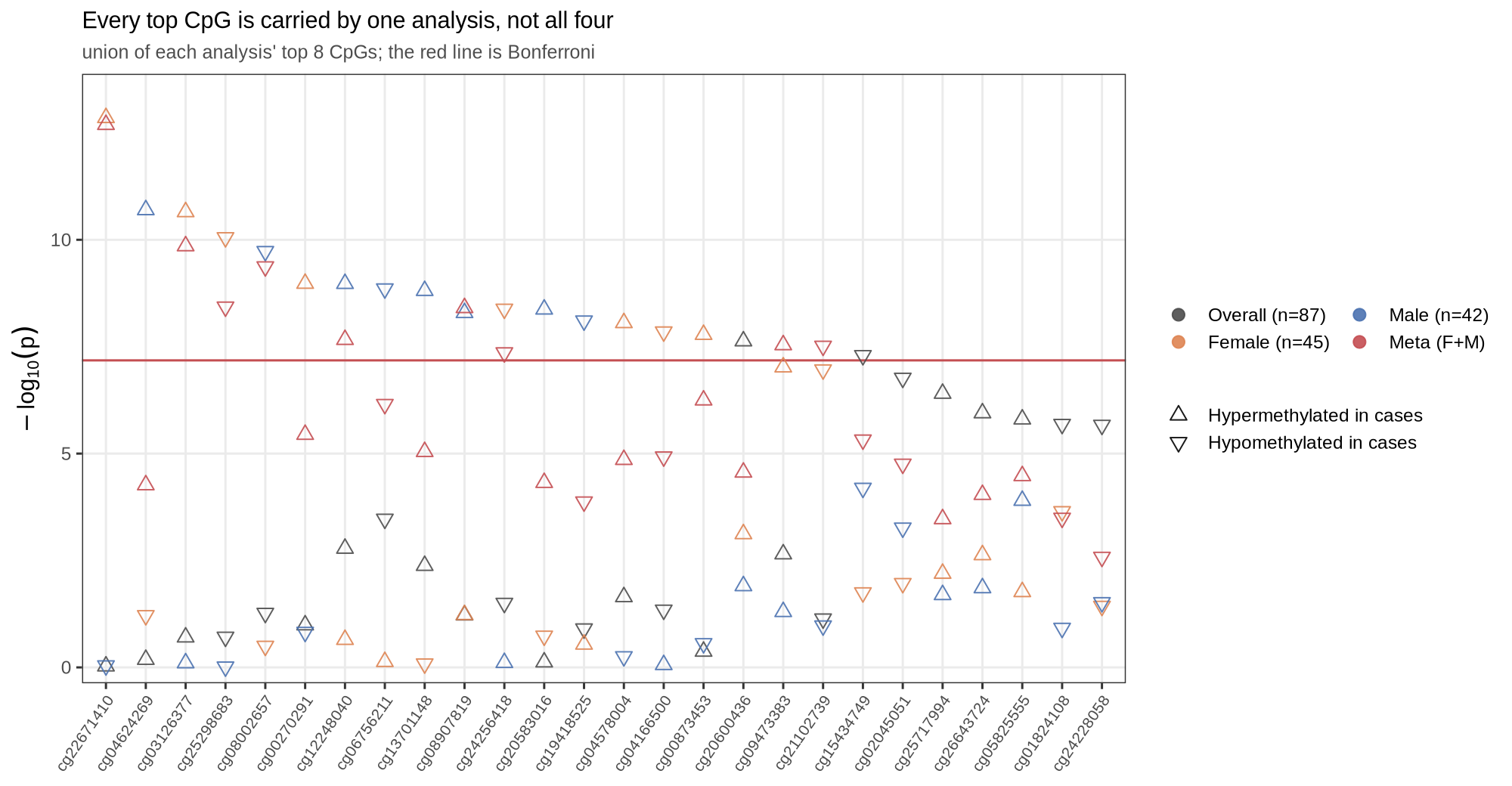
Ranking the union of each analysis's strongest CpGs makes the disagreement explicit:
{#fig-foothills}
Almost every CpG here is carried by a single analysis. Read across any column and you
typically find one point above the Bonferroni line and three well below it — the same
CpG, the same cohort, tested four ways, agreeing only occasionally. `cg22671410` is the
clearest case: top of the female arm and top of the meta-analysis, but essentially null
in the male arm and in the whole-cohort fit.
That is the pattern @fig-concordance quantifies for the nine meta-analysis hits:
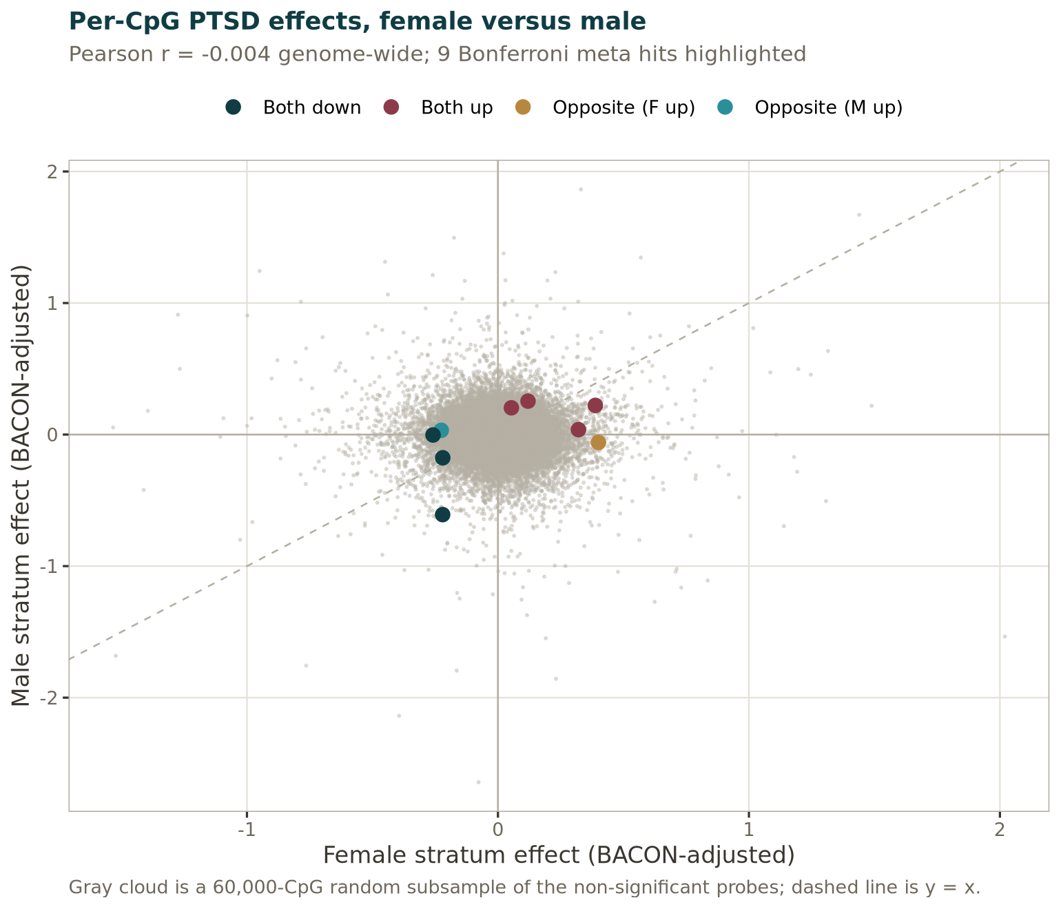{#fig-concordance width=70%}
A few caveats about these results:
- **The combined arm finds two CpGs at Bonferroni; the stratified arms and the
meta-analysis find many more.** The single-sex arms have an n that is too small to run
an EWAS. The sex-strata results prior to BACON adjustment were deflated and
inflated, and while BACON does adjust the stratum towards a lambda of 1,
respectively, it likely did not perform an optimal adjustment. The inflation
makes it appear as if there are statistically significant results where there
are none and is persisted in the meta-analysis results. This is not meant to be an
argument against doing stratified analyses, but it does bring to light the importance of
considering whether the sample size of your strata is sufficiently powered to do a stratified analysis.
- **Those two are not the same as chapter 06's one.** Both analyses call
`cg15434749`. The pipeline additionally calls `cg20600436`, and the two runs agree on
its effect estimate to seven decimal places (0.1717060) — they differ only in the
variance model. Its BACON p is 2.33 × 10⁻⁸ from the per-probe `glm` and
6.73 × 10⁻⁸ from `eBayes`, against a threshold of 6.61 × 10⁻⁸. The second value misses
by under 2%. A CpG this close to an arbitrary cutoff is likely a true result, 87 samples is
just too small to consistently detect it as genome-wide significant.
- **Heterogeneity sits at 5.4%** of CpGs below P = 0.05, against a 5% null
expectation, with a median I² of 0. There is no evidence of systematic
sex-differential methylation genome-wide. That does not mean that the heterogeneity
observed at the extremes is false, but with a sample size this small it does
warrant further investigation to validate if there are true sex differences at these sites.
The point of the chapter is
that the pipeline executes correctly, reproduces chapter 06's estimates to
floating-point precision, and produces calibrated statistics (λ within 2.5% of
1 in every arm). It is not that PTSD associates with these nine CpGs in 87
people.
## 10. Scaling up {#sec-scaling}
Nothing about the commands changes when you move from this demo to a real study —
you change `config.yml`, not the code:
- Point `mvals`/`pheno` at the full filtered matrix and sample table.
- Set `processing_type: cluster` and give Snakemake a cluster profile; the
chunking (`chunk_size`) turns each block of CpGs into a scheduler job.
- Add `dmr_analysis: "yes"` and the annotation settings to get region-level
results and gene annotation on top of the single-CpG output — which is what the
[next notebook](08_annotation.qmd) covers.
- Run `snakemake --cores N` (or `--profile <cluster>`) once, and every target in
the DAG — combined EWAS, stratified EWAS, BACON, METAL, DMRs, annotation,
plots — is built in order from a single reproducible entry point.
That is the payoff of the pipeline: the statistics are identical to what you did
by hand in chapter 06, but the *process* is now a versioned, parallel, one-command
artifact you can hand to a collaborator or a reviewer.
## References {.unnumbered}
::: {#refs}
:::


